Naive Bayes Outperforms Rivals in Audit Sampling of Financial, Text, and Network Data

Table of Links

• Abstract and 1. Introduction
• 2. Literature review
  • 3. Naive Bayes classifier
• 4. Results
  • 5. Discussion
  • 6. Conclusions and References

4. Results

This study generates three experiments to illustrate the benefits and limitations of combining a machine learning algorithm with sampling. The first experiment demonstrates that machine learning integration helps avoid sampling bias and maintains randomness and variability. The second experiment shows that the proposed works help sample unstructured data. The final experiment shows that the hybrid approach balances representativeness and riskiness in sampling audit evidence.

Referring to the previous study [15], implementing machine learning integration with sampling is better based on the accurate classification results provided by a machine learning algorithm. Therefore, this study chooses a random forest classifier and a support vector machines model with a radial basis function kernel as baseline models.

4.1. Experiment 1

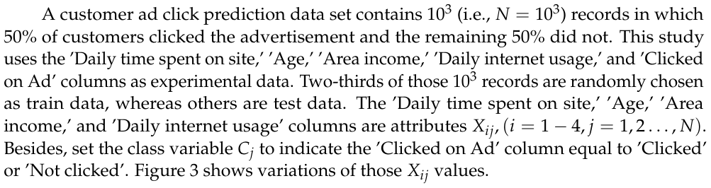
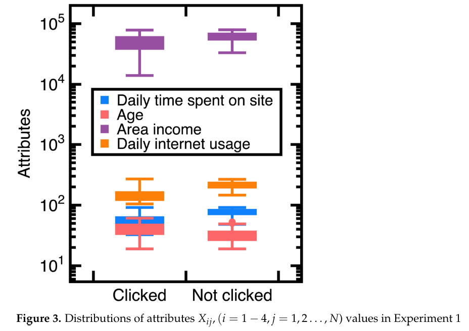
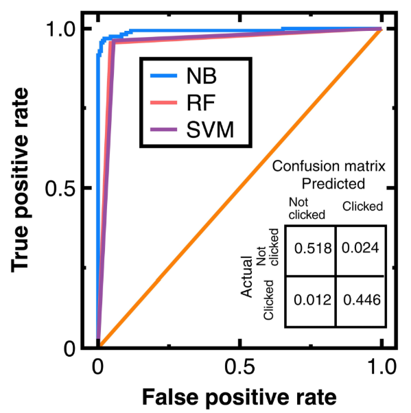
To avoid sampling frame errors [15], studying the classification accuracy output by Equations (3)-(4) is necessary. Figure 4 shows the resulting ROC curves in which NB, RF, and SVM are abbreviations of Naive Bayes, random forest, and support vector machines. This figure also shows the confusion matrix output by Equations (3)-(4). Its components have been normalized based on the amount of test data. Moreover, this study computes:

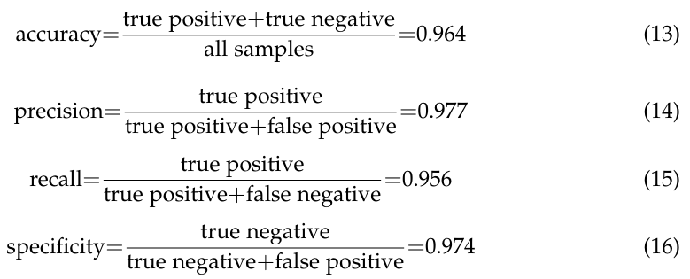
Further computing the F1 score from Equations (14)-(15) yields

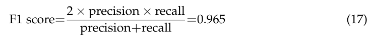
Meanwhile, calculating the AUC from Figure 4 obtains 0.965 (Equations (3)-(4)), 0.953 (Random forest classifier), and 0.955 (Support vector machines model with a radial basis function kernel). These AUC values indicate that Equations (3)-(4) slightly outperform the random forest classifier and support vector machines model with a radial basis function kernel in avoiding sampling frame errors and undercoverage. However, all three algorithms are good models.

Our aim for testing Section 3.1 is to sample an unbiased representation of experimental data with machine learning integration. Figure 5 shows the resulting audit evidence with a 50 % confidence interval for each class. Histograms on this figure’s top and right sides compare the distributions of original customers and audit evidence. In this figure, light and heavy gray points denote experimental data, whereas red and blue colors mark audit evidence. The total number of blue and red points in Figure 5 equal 250, respectively. Substituting the resulting audit evidence into Equation (7) obtains the representativeness indices RI listed in the legend of Figure 5.

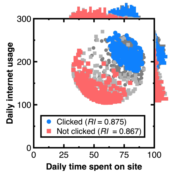
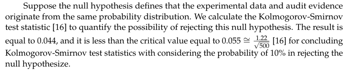
Calculating the Kolmogorov-Smirnov test statistic ensures that the audit evidence in Figure 5 is unbiased and representative of original customers. If the resulting KolmogorovSmirnov test statistic is lower than the critical value for concluding this test statistic, the original customers and audit evidence originate from the same probability distribution. Thus, we can reduce the risk of system errors or biases in estimating customers’ attributes.

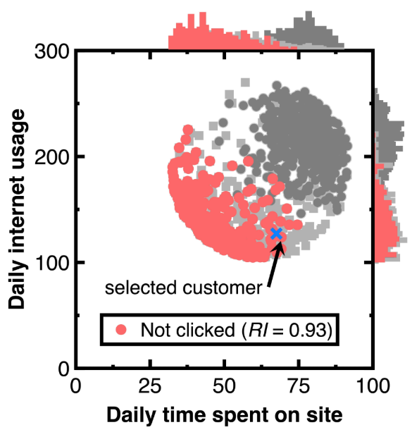
We have another aim of keeping the variability in testing Section 3.2. As marked by a blue cross in Figure 6, choose a customer with the predicted posterior probability of 0.999. The caption of Figure 6 lists the attributes of this customer. Other customers relevant to this customer are drawn as audit evidence and marked using red points in Figure 6. Besides, we still use light or heavy gray points representing the experimental data and histograms besides Figure 6 to describe the distribution of audit evidence. Since the denominator Pr(Ci) of Equation (11) equals 0.5. setting the σ2 threshold to 1.9999 is considered. Substituting the resulting audit evidence into Equation (7) yields the representativeness index RI in the legend of Figure 7. Counting the number of drawn audit evidence yields 294.

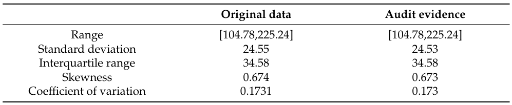
Table 1 compares variability between the original ’Daily Internet use’ variable and audit evidence. We employ the range, standard deviation, interquartile range, and coefficient of variation to measure the variability.

Measuring the variability helps understand the shape and spread of audit evidence. Table 1 shows that the audit evidence maintains the variability.

4.2. Experiment 2

A spam message is one of the unstructured data that did not appear in the conventional sampling. In this experiment, this study introduces a data set containing 5572 messages, and 13 % of them are spam. This study randomly selects 75 % of them as train data. The other 25 % are test data. In implementing this experiment, the first step is preprocessing these train and test data by vectorizing each message into a series of keywords. We employ a dictionary to select candidate keywords. Counting their frequencies is next performed. Classifying ham and spam messages is done by setting a class variable Ci (1 ≤ i ≤ N) indicating a spam or ham message, and attributes are the frequency of keywords.

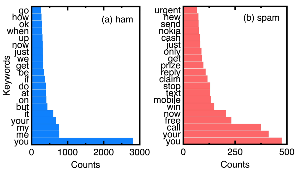
Based on the counts of keywords in ham and spam messages of experimental data, Figure 7 compares the top 20 keywords. Choosing them eliminates ordinary conjunctions and prepositions such as ’to’ and ’and.’ We can understand the unique keywords of spam messages from Figure 7.

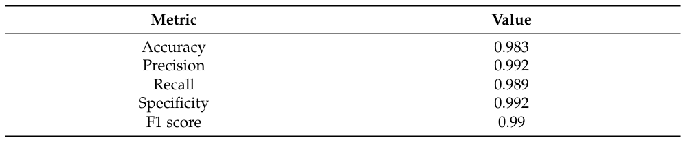
To prevent sampling frame errors and undercoverage [15], Figure 8 compares the corresponding ROC curves versus different machine learning algorithms. It also shows the confusion matrix output by Equations (3)-(4). We have normalized its components based on the amount of test data. Table 2 lists other metrics for demonstrating classification accuracy on this confusion matrix.

Calculating the AUC values from Figure 8 yields 0.989 (Equations (3)-(4)), 0.923 (Random forest classifier), and 0.934 (Support vector machines model with a radial basis function kernel). Such AUC values indicate a support vector machines model, random forest, and Equations (3)-(4) are all good models for preventing sampling frame errors and undercoverage; however, the performance of Equations (3)-(4) is still the best.

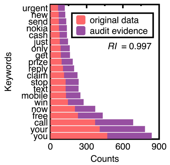
Next, this study chooses the 75 % confidence interval of spam messages to generate audit evidence. We obtained 652 samples of spam messages. Figure 9 compares counts of the top 20 keywords of original text data and audit evidence. Substituting their posterior probabilities to compute the representativeness index RI equals 0.997.

Figure 9 demonstrates that machine learning integration promotes sampling unstructured data (e.g., spam messages) while keeping their crucial information. The design of conventional sampling methods does not consider unstructured data [4]. In this figure, sampling spam messages keeps the ranking of all the top 20 keywords. The resulting samples may form a benchmark data set for testing the performance of different spam message detection methods.

4.3. Experiment 3

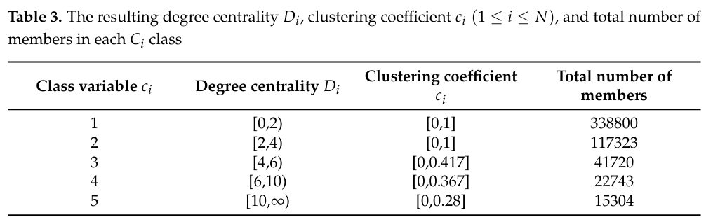
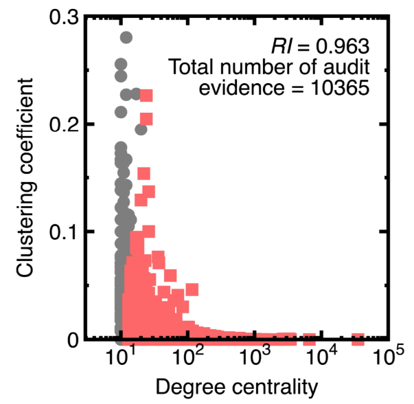
The third experiment illustrates that integrating machine learning with sampling can balance representativeness and riskiness. We use the Panama Papers to create a directed graph model having 535891 vertices in which each vertex denotes a suspicious financial account. Its attributes are the degree centrality and clustering coefficient.

The Panama Papers were a massive leak of documents. They exposed how wealthy individuals, politicians, and public figures worldwide used offshore financial accounts and shell companies to evade taxes, launder money, and engage in other illegal activities.

The degree centrality D [17] is the number of edges connecting to a vertex. The higher the degree centrality, the greater the possibility detects black money flows. Besides, we consider that two financial accounts may have repeated money transfers. Therefore, computing the degree centrality considers the existence of multiple edges. For example, if a sender transfers money to a payee two times, the degree of a vertex simulating such a sender or payee equals 2.

Meanwhile, the clustering coefficient c [17] measures the degree to which nodes in a graph tend to group. Evidence shows that in real-world networks, vertices may create close groups characterized by a relatively high density of ties. In a money laundering problem, a unique clustering coefficient may highlight a group within which its members exchange black money. Like the computation of degree centrality, calculating the clustering coefficient considers the possible existence of multiple edges.

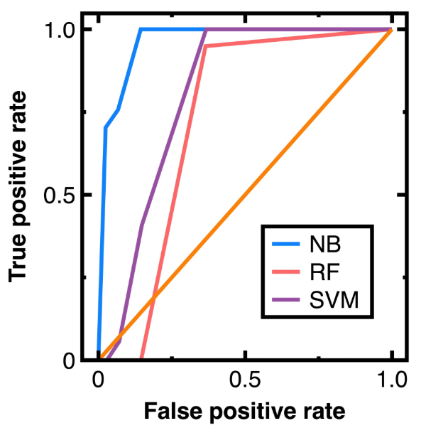
To prevent sampling frame errors and undercoverage [15], Figure 10 compares the ROC curves output by different machine learning algorithms in classifying nodes in Experiment 3. Obtaining Figure 10 chooses 80 % of random nodes as train data and other vertices as test data. Moreover, Equations (3)-(4) output the confusion matrix shown in Equation (18):

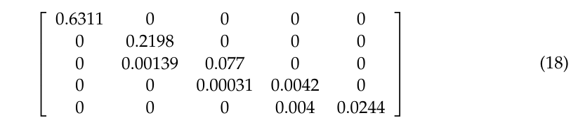
in which each component has been normalized based on the amount of test data.

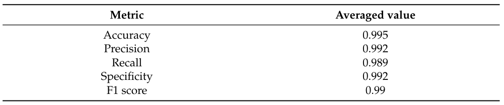
From Equation (18), we further calculate the averaged accuracy, specificity, recall, precision, and F1 value, as shown in Table 4. Next, calculating the AUC values from Figure 10 and Table 4 results in 0.965 (Equations (3)-(4)), 0.844 (Random forest classifier), and 0.866 (Support vector machines model with a radial basis function kernel). Figure 10 indicates that the random forest classifier and support vector machines model with a radial basis function kernel are unsuitable for this experiment. Since we have a high volume of data in this experiment, these two algorithms may output unacceptable errors in sampling nodes.

5. Discussion

Section 4 implies the benefits and limitations of integrating a Naive Bayes classifier with sampling. We further list these benefits and limitations:

• Conventional sampling methods [4] may not profile the full diversity of data; thus, they may provide biased samples. Since this study samples data after classifying them using a Naive Bayes classifier, it substitutes for a sampling method to profile the whole diversity of data. Experimental results of Section 4 indicate that the Naive Bayes classifier classifies three open data sets accurately, even if they are excessive. Those accurate classification results indicate that we capture the whole diversity of experimental data.

• Developing conventional sampling methods may not consider complex patterns or correlations in data [4]. In this study, we handle complex correlations or patterns in data (for example, a graph structure in Section 4.3) by a Naive Bayes classifier. This design mitigates the sampling bias caused by complex patterns or correlations if it provides accurate classification results.

• Section 4.3 indicates that a Naive Bayes classifier works well for big data in a money laundering problem. It outperforms the random forest classifier and support vector machines model with a radial basis function kernel in classifying massive vertices. Thus, we illustrate that the efficiency of sampling big data can be improved. One can sample risker nodes modeling fraudulent financial accounts without profiling specific groups of nodes.

• Development of conventional sampling methods considers structured data; however, they struggled to handle unstructured data such as spam messages in Section 4.2. We resolve this difficulty by employing a Naive Bayes classifier before sampling.

• Since this study samples data from each class classified by a Naive Bayes classifier, accurate classification results eliminate sample frame errors and improper sampling sizes.

Nevertheless, this study also finds limitations in integrating machine learning and sampling. They are listed as follows:

• It is still possible that a Naive Bayes classifier provides inaccurate classification results. One should test the classification accuracy before sampling with machine learning integration.

• In implementing Section 3.2, thresholds σj (j = 1−3) are needed. However, we should inspect variations of the prior probabilities for determining proper σj (j = 1 − 3) values. They denote the second limitation of our machine learning-based sampling.